
Tokenization and Embeddings
A computer stores text as a string of characters, yet a model that predicts text cannot work on the unlimited set of all strings, so the first job is to cut text into pieces drawn from a fixed list and turn each piece into numbers. A language model is a program that reads some text and assigns a probability to each possible next piece. Each piece is a token, which can be a whole common word, a fragment of a rarer word, or a single byte. The program that does the cutting is the tokenizer, and the fixed list of pieces it may emit is the vocabulary, with every piece numbered by an integer id.
Two separate decisions hide inside “turn text into numbers”, and people often blur them. The tokenizer decides where the cuts go, which fixes how many tokens a document costs and which strings the model can ever see as one unit. The embedding table then gives each token id one row of learned numbers, called its embedding, and those rows are what the rest of the network actually computes with. The figure cuts one sentence three ways to show what the first decision trades.
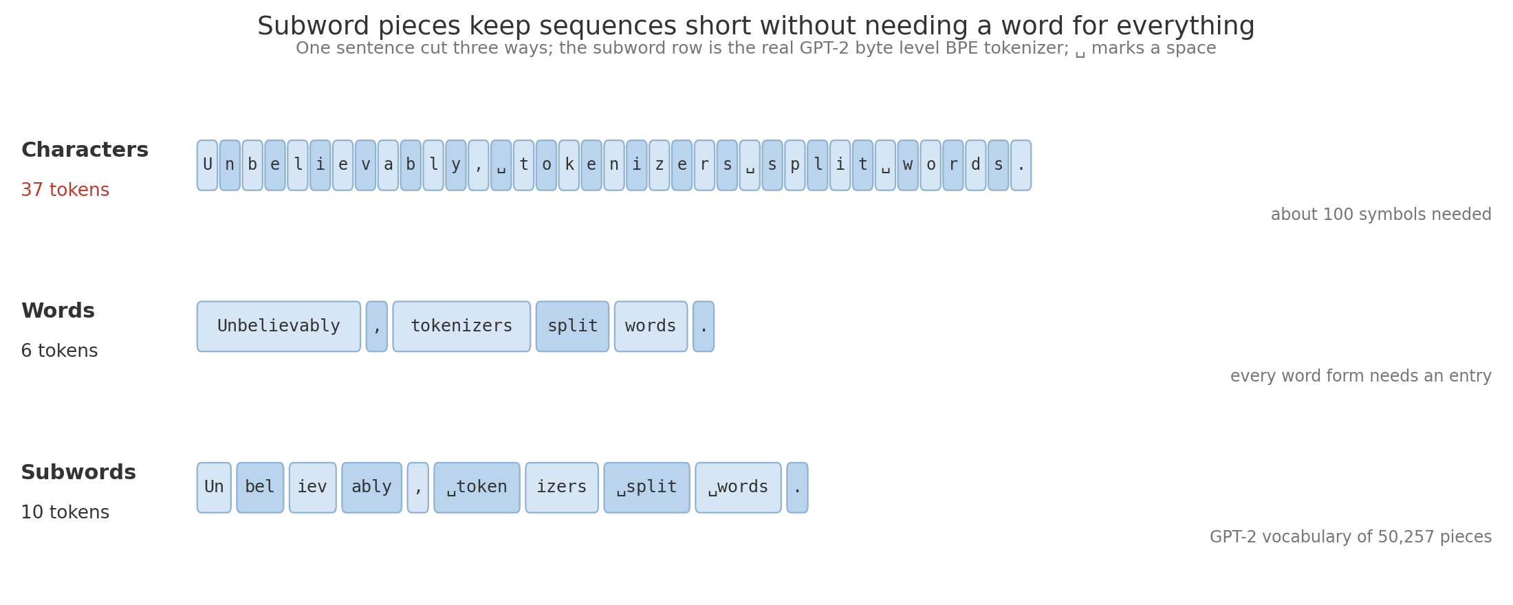
Characters give long sequences from a tiny list, words give short sequences from a list that can never be complete, and subword pieces sit between them. Almost every design question in this note is a question about where on that line to stand, and what it costs in table size, sequence length, and the strings a model can no longer see inside.
1. The choice of text unit
Section titled “1. The choice of text unit”Before any learning happens, someone has to decide what counts as one unit of text. Think of reading a phone number aloud: you can say it digit by digit, or in chunks such as “five five five, one two three four”, and the chunked version is shorter but needs you to know more chunk names. A tokenizer has to make the same trade-off between two costs. One is the sequence length , the number of tokens a text becomes. The other is the size of the vocabulary, the list of pieces the model must know. Making the pieces bigger shortens the sequence but lengthens the list, and making them smaller does the reverse.
Characters need only about a hundred symbols for English, so nothing is ever missing, but the opening sentence “Unbelievably, tokenizers split words.” becomes 37 tokens. Length is expensive because attention, the step in which every position compares itself with every earlier position (developed in Attention and Positional Information), does work that grows with , so 37 tokens mean about 1,369 position pairs where 10 tokens mean 100. Length also eats the context window, the maximum number of tokens the model can read at once, which is 4,096 in the reference model. At roughly 5.7 characters per English word including the space, 4,096 characters hold about 720 words.
Splitting on whole words turns the same sentence into just 6 tokens, far shorter than 37. The problem is that no list of words is ever complete. English alone has hundreds of thousands of word forms, and real text also contains names, typos, numbers and code identifiers, so words outside any fixed list keep appearing. A word-level model has to replace each of them with one shared placeholder, the unknown token, usually written <unk>. After that replacement, a name such as “Okonkwo”, a typo such as “recieve”, and a code name such as “x_train” all reach the model as the same id, so it cannot tell them apart or learn anything about any of them.
A subword vocabulary keeps frequent words whole and builds rare ones from smaller pieces. GPT-2’s tokenizer, with 50,257 pieces, keeps ” split” and ” words” whole and builds “Unbelievably” from “Un”, “bel”, “iev” and “ably”, for 10 tokens in total. On ordinary English chat text a 32,000 piece vocabulary averages about 1.3 tokens per word (measured in section 5), so the same 4,096 token context holds roughly 3,100 words instead of 720. Every modern large language model, abbreviated LLM, uses some form of subword tokenizer.
2. Byte pair encoding
Section titled “2. Byte pair encoding”The most common way to choose subword pieces is to let frequency decide. If “th” shows up constantly in English, it is worth giving it its own symbol, and once “th” exists, “the” may become worth a symbol too. Byte pair encoding, abbreviated BPE, applies that idea greedily, and Sennrich et al. brought it from data compression to machine translation in 2016.
The name comes from that compression origin. Philip Gage’s 1994 method shrank a file by finding the pair of adjacent bytes that occurred most often, replacing every copy with one unused byte, and repeating. A tokenizer uses the same loop for a different goal. Each new symbol it creates shortens every text that contains the pair, so the pieces it ends up with are the ones that save the most tokens on typical text.
Training a BPE tokenizer starts with every word split into single characters. It then counts every adjacent pair of symbols in the training corpus, the sample of text the tokenizer learns from, weighting each pair by how often its word appears. The most frequent pair becomes one new symbol through a merge, every occurrence in the corpus is rewritten, and the counting repeats until the vocabulary reaches the target size . The output is the merge list, the ordered sequence of merges, and that list together with the base characters is the whole tokenizer. Before any counting, the text is cut into words by a fixed rule, a step called pre-tokenization. Merges are only allowed inside these words, so a token never spans two words and the tokenizer does not waste entries on frequent phrases such as “of the”. Spaces are kept rather than thrown away, because the model has to reproduce them when it writes text. GPT-2’s tokenizer attaches each space to the word after it and prints it as Ġ, so ” the” and “the” are different tokens, while SentencePiece, a tokenizer library used by Llama, writes the space as ▁. Counting each distinct word once and multiplying by its frequency is also what makes training fast enough, since a large corpus has billions of words but far fewer distinct ones.
The algorithm step by step
Section titled “The algorithm step by step”Written as a procedure, BPE has two parts. Training reads a corpus once and learns the merge list. Encoding, turning new text into tokens with a finished tokenizer, uses that fixed list to turn any new text into token ids. In Algorithm 1, is the training corpus, the base symbols, which are characters in the example below and bytes in real tokenizers, the merge list, how often word occurs, and how many times symbol is directly followed by symbol inside , so is the pair count weighted by word frequency.
To see each line operate, run Algorithm 1 on a corpus of four words with counts low ×5, lower ×2, lowest ×3 and newest ×6, with target . Lines 1 and 2 split every word into characters, which gives the 8 base symbols l, o, w, e, r, s, t and n. When two pairs tie at line 6, the rule here is to take the pair met first when reading the words in that listed order. Each row of the table is one pass through lines 4 to 8, with the four largest pair counts from line 4.
| Round | Line 4, largest pair counts | Line 6, merge | Line 8, the four words afterwards | Vocabulary |
|---|---|---|---|---|
| 1 | w e 11, l o 10, o w 10, e s 9 | w + e → we | l o w, l o we r, l o we s t, n e we s t | 9 |
| 2 | l o 10, we s 9, s t 9, n e 6 | l + o → lo | lo w, lo we r, lo we s t, n e we s t | 10 |
| 3 | we s 9, s t 9, n e 6, e we 6 | we + s → wes | lo w, lo we r, lo wes t, n e wes t | 11 |
| 4 | wes t 9, n e 6, e wes 6, lo w 5 | wes + t → west | lo w, lo we r, lo west, n e west | 12 |
| 5 | n e 6, e west 6, lo w 5, lo west 3 | n + e → ne | lo w, lo we r, lo west, ne west | 13 |
| 6 | ne west 6, lo w 5, lo west 3, lo we 2 | ne + west → newest | lo w, lo we r, lo west, newest | 14 |
| 7 | lo w 5, lo west 3, lo we 2, we r 2 | lo + w → low | low, lo we r, lo west, newest | 15 |
Round 1 counts w e as , once each from lower, lowest and newest, which beats l o and o w at 10. Round 2 shows why line 4 recounts after every merge. The pair o w counted 10 in round 1 but only 5 in round 2, because merge 1 used up the w inside lower and lowest. Rounds 3 and 5 are ties that line 6 settles by order, we s over s t at 9 and n e over e west at 6. After round 7 the vocabulary has 15 symbols, so line 3 stops the loop and the merge list holds seven pairs.
Encoding needs no counts at all, only the merge list. In Algorithm 2, is the new text to tokenize.
Now run Algorithm 2 on “slowest”, a word the training corpus never contained, using the seven merges above numbered 1 to 7 in the order they were learned. Line 3 splits it into s l o w e s t. Each row is one pass of the loop in lines 4 to 6, listing the pairs of the word that appear in the merge list, with their merge numbers.
| Pass | Line 4, pairs found in the merge list | Line 5, earliest | Line 6, the word afterwards |
|---|---|---|---|
| 1 | l o (2), w e (1) | w e (1) | s l o we s t |
| 2 | l o (2), we s (3) | l o (2) | s lo we s t |
| 3 | we s (3) | we s (3) | s lo wes t |
| 4 | wes t (4) | wes t (4) | s lo west |
| 5 | none | the loop ends | s lo west |
Line 7 then outputs the ids of s, lo and west, three tokens and no unknown token, even though the word never appeared in training. Merge 7, lo + w, never fires, because merge 1 already joined w to e. Merges 5 and 6 never fire either, since “slowest” has no n.
Real implementations of training do not recount every pair after each merge. They keep the pair counts and update only the words that contained the merged pair, which is what lets a tokenizer with tens of thousands of merges train on billions of words.
What the run shows
Section titled “What the run shows”After 7 merges the vocabulary has 8 + 7 = 15 symbols. The word low and the word newest are each one token, lowest is lo + west, and lower is lo + we + r. The pieces follow frequency and have nothing to do with meaning, which is why “west” appears inside “lowest”.
The run also shows why merging the most frequent pair is the right greedy choice. A merge with weighted count turns pairs of symbols into single symbols, so it shortens the corpus by exactly tokens. The corpus starts as characters. The seven merges have counts 11, 10, 9, 9, 6, 6 and 5, which add up to 56, so the corpus ends at tokens, the same as counting the final pieces word by word: 5 for low, for lower, for lowest and 6 for newest. Picking the largest count at each step gives the biggest saving available at that step. It does not guarantee the best possible vocabulary overall, since an early merge can block a later one, the way “we” stopped “low” from forming inside “lower”.
The animation replays the seven training rounds with their pair counts and then the encoding of “slowest”. Training and encoding differ in what they cost and what they depend on. Training counts pairs over a large corpus once, while encoding only applies a fixed list, so the same string always gets the same tokens. Production tokenizers implement encoding by repeatedly applying the earliest learned merge present in the word, which gives the same result as this replay. A real 32,000 entry vocabulary built on 256 base bytes holds 31,744 merges.
Real tokenizers change three details of this toy version. First, the base symbols are usually the 256 possible byte values rather than letters, which is called byte-level BPE and means any string at all can be encoded, as section 4 explains. Second, many tokenizers add rules for digits. On ” the lowest price is 12345”, GPT-2’s tokenizer gives Ġthe, Ġlowest, Ġprice, Ġis, Ġ123 and 45, splitting the number wherever its merges happen to stop, while the SmolLM2 tokenizer splits every digit into its own token, as Llama does, so numbers are always cut the same way. Third, the training corpus decides everything. A tokenizer trained mostly on English text learns long English pieces and cuts other languages and code into many short ones, which is the cost section 6 measures, and it splits a rare word wherever its frequent fragments are, as with “photos” and “ynthesis” for “photosynthesis” in 15a.
3. WordPiece and Unigram tokenizers
Section titled “3. WordPiece and Unigram tokenizers”Byte pair encoding merges whatever pair is most common, but a common pair is not always a meaningful one. Two very frequent letters will sit next to each other often just by chance, the way “e” and “s” do in English, while a pair such as “q” and “u” almost never appears apart. Two other tokenizer families score candidate pieces with probabilities instead of raw counts.
WordPiece, used by BERT (Devlin et al.) with a vocabulary of about 30,000, keeps the merging of small pieces from byte pair encoding (BPE) into larger ones but scores a pair by how much more often it occurs than chance would predict.
Here is the count of the pair and and are the counts of each symbol on its own. Choosing the highest score approximately maximizes the likelihood of the corpus, meaning the probability a simple model built from the pieces assigns to the whole training text. On the corpus from section 2 the letter counts are , , and . The pair s t scores , the highest of any pair, because s is never seen without t. The pair w e that BPE merged first scores only , since both letters are common everywhere. WordPiece marks a piece that continues a word with ##, so a WordPiece tokenizer splits “tokenization” into token and ##ization.
A Unigram tokenizer (Kudo) works in the opposite direction. It starts from a large candidate vocabulary, gives each piece a probability , and segments a word into the pieces whose probabilities multiply to the largest value. Suppose , , and , and every single letter has probability 0.02. Then low + est scores , lo + west scores , and six single letters score , so the tokenizer picks low + est. Training alternates between re-estimating these probabilities and pruning, removing the pieces whose loss would lower the corpus likelihood least, until the vocabulary shrinks to the target size.
SentencePiece (Kudo and Richardson) is a library that runs BPE or Unigram directly on raw text, treating the space as an ordinary symbol written ▁. “Hello world” becomes ▁Hello and ▁world, so decoding is exact and the tokenizer needs no rule about where words begin, which matters for Chinese, Japanese and Thai, written without spaces. Llama 2’s 32,000 entry tokenizer is SentencePiece BPE (Touvron et al.).
4. Byte level fallback
Section titled “4. Byte level fallback”Even a large subword vocabulary will meet a character it has never seen, such as a rare Chinese character, an emoji, or a symbol from a math paper. A tokenizer needs some way to write such characters down without giving up and emitting an unknown token. The answer is to fall back to the raw bytes the computer already uses to store the text.
A byte is a number from 0 to 255, so there are exactly 256 of them. UTF-8 is the standard rule for storing any character as one to four bytes, and the figure shows the actual bytes. The letter a is the single byte 61 in hexadecimal, é takes 2 bytes, the Chinese character 東 takes 3, and the emoji 😀 takes 4. Any text, in any script, is therefore a sequence of those 256 values.
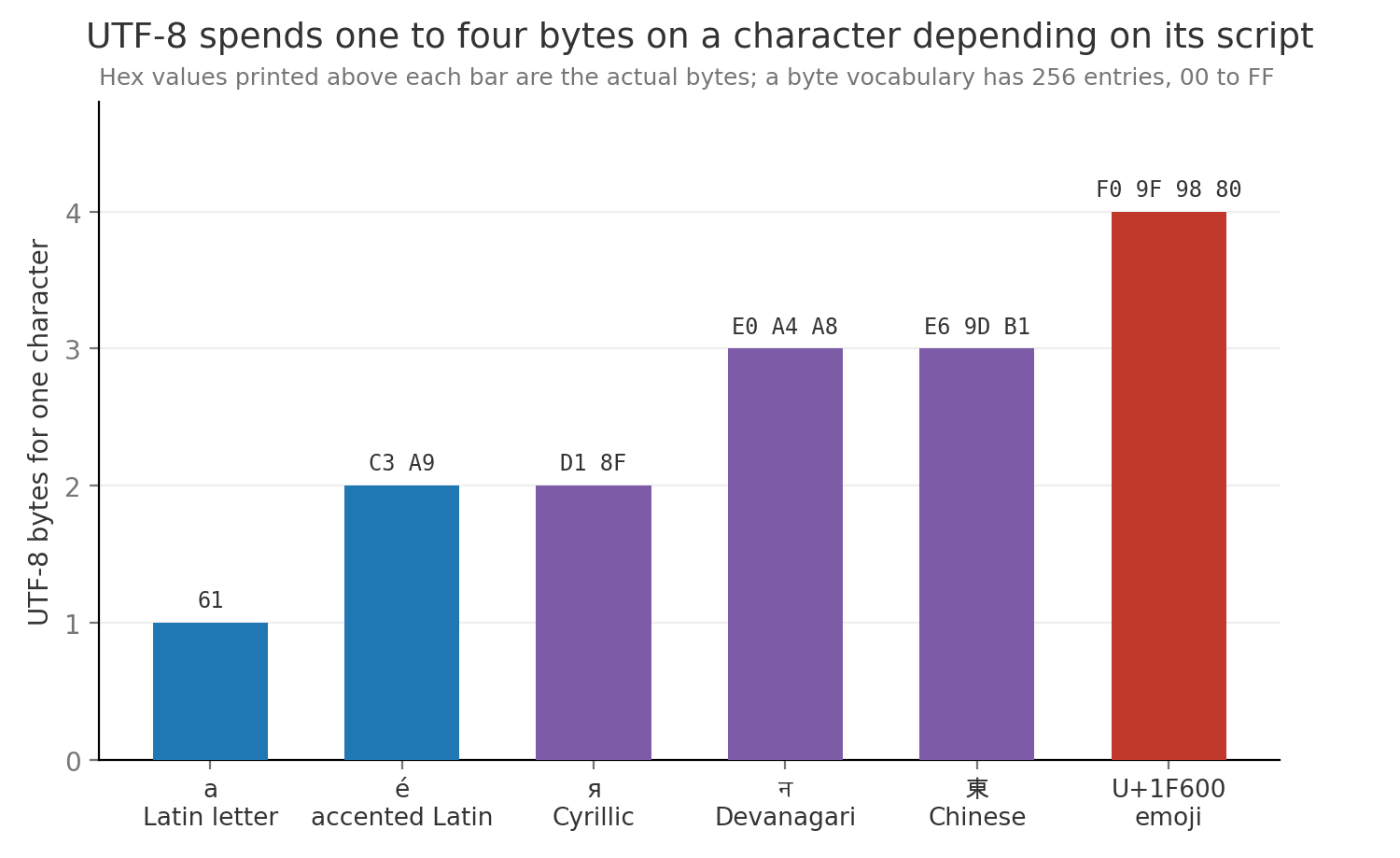
Two designs use this. Byte fallback, used by Llama 2, keeps the 256 byte values as reserved vocabulary entries and spells any character that has no piece as its UTF-8 bytes, so a missing 東 costs 3 tokens instead of one unknown token. Byte level BPE, introduced with GPT-2 (Radford et al.), goes further and runs byte pair encoding on bytes from the start, so the 256 bytes are the base alphabet and every merge combines bytes. GPT-2’s tokenizer turns ” 東京”, a space and two characters stored in 7 bytes, into 5 tokens, several of which are fragments of a character that print as � on their own.
Both designs guarantee that every string can be encoded and decoded back exactly. They do not guarantee that the model handles the string well, because a character spelled out as three rare byte tokens arrives as pieces the model has seen little of during training, and it makes the text longer. That length cost is the subject of section 6.
5. Vocabulary size tradeoff
Section titled “5. Vocabulary size tradeoff”A bigger vocabulary lets more strings become single tokens, the way a person with a larger vocabulary can say “photosynthesis” instead of describing it. The price is paid in two tables that grow with every entry. The embedding table has rows of numbers. The output head is the matrix at the end of the model that turns the final hidden vector into one score per vocabulary entry, so it also has rows of numbers. Each score is a logit , a raw number that a softmax later turns into a probability (see Language Modeling and Next Token Prediction).
A parameter is one learned number in the model. In the reference model the two tables are separate, so each holds parameters and together they hold 262,144,000, about 3.9% of the 6.74 billion total. Growing to 128,000 entries makes each table , so the pair grows by 786,432,000 and the model reaches about 7.52 billion parameters with an unchanged body.
Compute changes in two opposite directions. A floating point operation, or FLOP, is one multiplication or addition, and a forward pass costs about two FLOPs per parameter per token. Reading a row of costs no arithmetic, but the output head costs FLOPs per token, which is 262,144,000 at 32,000 and 1,048,576,000 at 128,000. The body of the reference model, everything except the two tables, has 6,476,271,616 parameters and costs about 12.95 billion FLOPs per token, so each token costs about 13.21 billion FLOPs at 32,000 and 14.00 billion at 128,000, about 6% more.
The 32,000 against 128,000 comparison
Section titled “The 32,000 against 128,000 comparison”The steps below decide between a 32,000-token and a 128,000-token vocabulary for the reference 7B model. They measure how many tokens each needs per word, price the same 1,000 words both ways, and then add the costs that a FLOP count misses.
- Measure tokens per word. On held out chat text, byte pair encoding tokenizers trained on 106 MB of the same text produce 1.316 tokens per word at 32,000 and 1.261 at 128,000, about 4% fewer. Meta reports up to 15% fewer tokens for Llama 3’s 128,000 entry vocabulary than for Llama 2’s on its own data (Llama 3), because a web scale corpus has many more strings frequent enough to deserve a merge.
- Price 1,000 words at the measured rate. At 32,000 that is billion, about 17.4 trillion FLOPs. At 128,000 it is billion, about 17.7 trillion, so the bigger vocabulary costs 1.5% more.
- Price it at Meta’s rate. With 15% fewer tokens the bigger vocabulary costs of the smaller one, a saving of about 10%. The direction of the result depends on how much shorter the text really gets.
- Add the memory that FLOPs miss. During training the logits for a 4,096 token sequence stored as 4 byte numbers take bytes, about 0.52 GB, at 32,000 and about 2.10 GB at 128,000, per sequence.
- Add the statistical cost. With four times as many entries, each rare entry appears in fewer training examples, so its row of receives fewer updates and stays closer to its random starting values.
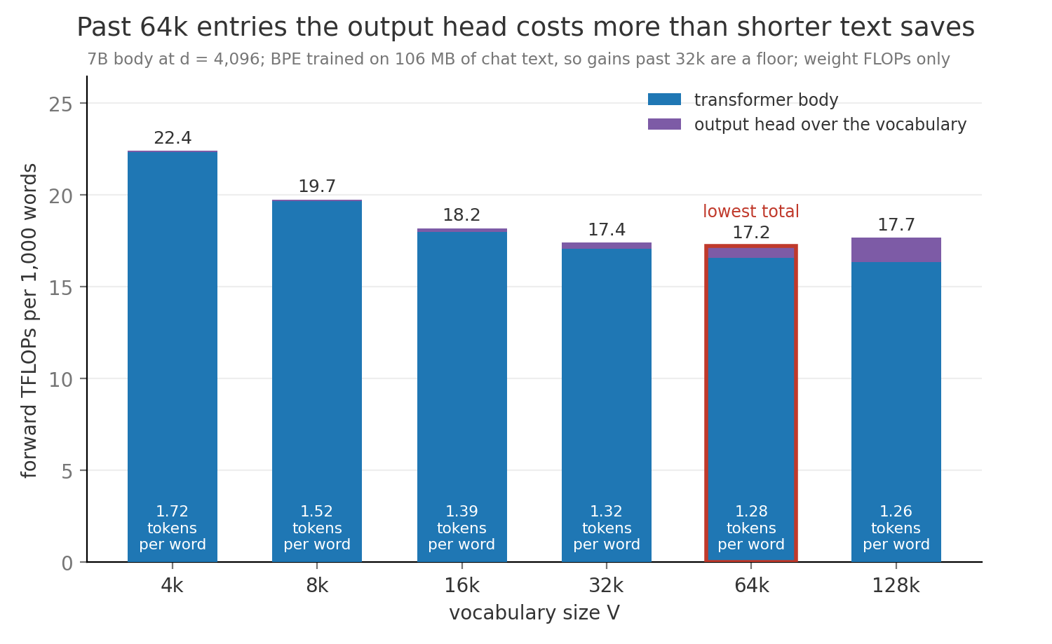
The figure runs the same arithmetic across six vocabulary sizes on the small corpus. Total compute falls quickly from 4,000 to 32,000 entries, flattens, and on this corpus turns up after 64,000, because the head keeps growing in proportion to while the token savings shrink. Shorter sequences also save attention work and context space that the figure leaves out, which is one reason recent multilingual models choose 128,000 to 256,000 entries. A larger model width shrinks the tables’ share of parameters, so a 1B model pays relatively more for the same vocabulary than a 70B model.
6. Fertility across languages
Section titled “6. Fertility across languages”A tokenizer learns its pieces from its training corpus, so it learns long pieces for the languages that dominate that corpus. Think of a phrasebook written for English speakers that has whole sentences for English and only an alphabet chart for Hindi, so every Hindi sentence has to be spelled out letter by letter. Fertility is the average number of tokens per word for one language under one tokenizer, and it is the number that captures how far a language is from that phrasebook ideal.
The figure tokenizes one sentence, “The doctor said the test results will be ready next week”, and its translations with two real tokenizers. GPT-2’s vocabulary was trained on mostly English text, and it spends 12 tokens on the English sentence, a fertility of about 1.1 for its 11 words, but 79 tokens on Russian and 94 on Hindi, 6.6 and 7.8 times the English count. Qwen2.5’s vocabulary of 151,665 pieces was trained on multilingual text and spends 20 tokens on Russian and 58 on Hindi. It spends only 8 on Chinese, fewer than on English, because it learned whole Chinese words as single pieces.
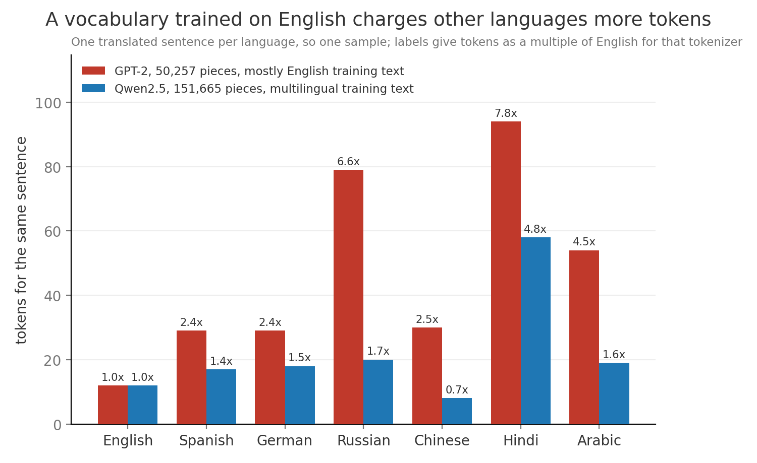
The ratio of a language’s token count to English for the same meaning is sometimes called its token premium, and Petrov et al. measured premiums above 10 for some language and tokenizer pairs. With the GPT-2 figure for Hindi, three costs follow for the reference model. A 4,096 token context holds only as much Hindi as English would fill in about 525 tokens. Decoding at batch 1 runs at about 4.0 ms per token, so an answer that takes 130 tokens in English, about 0.52 seconds, takes about 1,014 tokens and 4.1 seconds in Hindi. An application programming interface, or API, billed per token charges the Hindi user about 7.8 times as much for the same content. One sentence is a small sample, so measure fertility on real traffic in each language before quoting a number.
7. Special tokens and chat templates
Section titled “7. Special tokens and chat templates”A model reading a conversation needs to know where one message ends and the next begins, and who wrote each one, much as a screenplay labels each speaker before their lines. Plain text has no reliable markers for that, so tokenizers reserve a few ids that never come from ordinary text. These are special tokens, each a single id with a fixed job.
The common ones are the beginning of sequence token, abbreviated BOS and written <s> in Llama 2, which marks the start of a document, and the end of sequence token, abbreviated EOS and written </s>, which the model learns to emit when it is finished, so generation stops there. A padding token fills unused positions when sequences of different lengths are stacked into one batch, and it is excluded from the loss. Chat models add role markers, special tokens that announce a system, user or assistant message.
A chat template is the exact rule that turns a list of messages into one token sequence, including the role markers, the newlines between them and the place where the assistant’s reply starts. Qwen2.5 uses the ChatML template, and the figure shows a three message conversation becoming 26 tokens, 6 of which are single special tokens such as <|im_start|>. The same conversation written in Llama 2’s [INST] format and sent to Qwen2.5 becomes 29 tokens with no special tokens at all, because [INST] and <<SYS>> are not entries in Qwen’s vocabulary and get split into ordinary pieces such as [, INST and ].
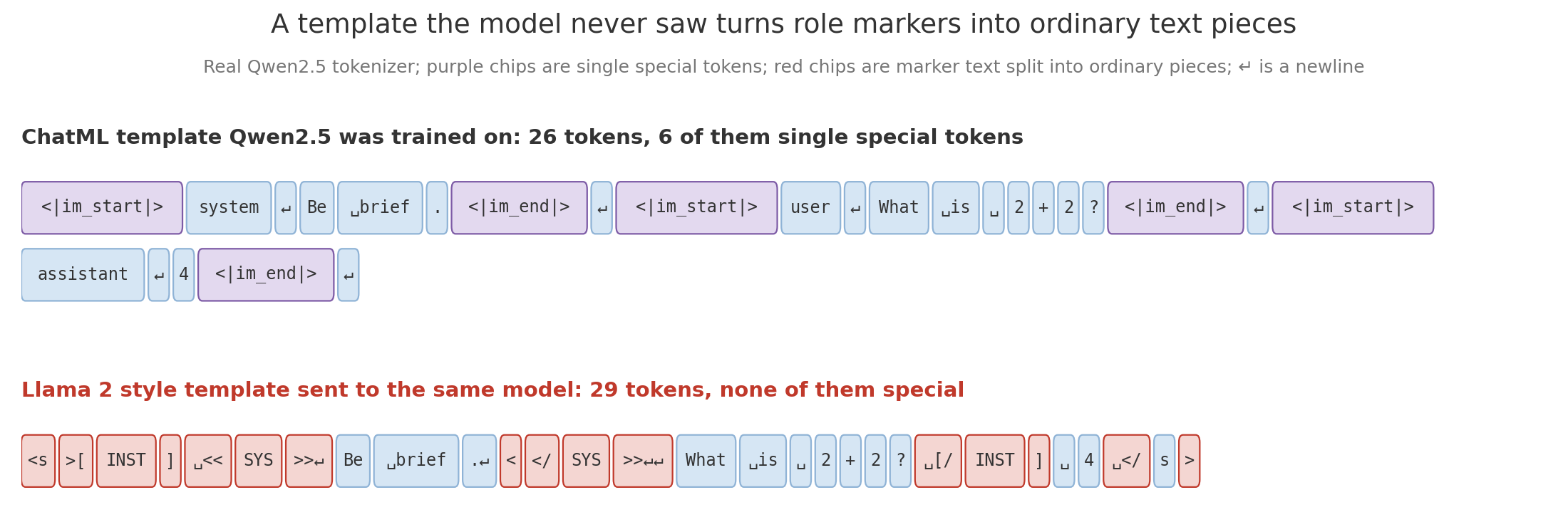
The model learned the meaning of its role markers during fine-tuning, the extra training on conversations that turns a raw text predictor into an assistant (see Post Training from Base Model to Assistant). With the wrong template the markers it relies on are absent, so it sees a conversation shaped like no example it was trained on. Nothing raises an error, since every string still tokenizes. Instead quality drops quietly: the model may ignore the system message, continue writing the user’s turn, or never emit its end token and keep generating. Smaller mismatches do the same damage, such as a missing newline after the assistant marker, a BOS token added twice, or a fine-tuning set formatted with one template and served with another.
8. Embedding lookup
Section titled “8. Embedding lookup”Once text is a list of token ids, the network needs numbers it can compute with, and an id such as 1,532 carries no meaning as a quantity, since token 1,532 is not “more” than token 1,531. A library catalogue works the same way: the call number tells you which shelf to visit, and the book on that shelf holds the content. Embedding lookup uses the token id the same way, as the index of a row in the embedding table , and returns that row as the token’s vector of numbers.
The lookup can be written as a matrix product, which is how it fits into the same algebra as the rest of the network. A one-hot vector has entries, 1 in position and 0 elsewhere. Multiplying it by gives , since each output coordinate adds up one-hot entries times table entries and only the entry for token is nonzero.
A lookup computed both ways
Section titled “A lookup computed both ways”The steps below take a five-token vocabulary and fetch one token’s embedding twice, once as a row lookup and once as a one-hot vector multiplied by the table. Both give the same vector, which is why real models use the cheap lookup.
- Take a vocabulary of 5 tokens with ids 0 to 4, namely the, cat, sat, on and mat, and width . The table rows are the (0.1, 0.3, −0.2), cat (0.7, −0.4, 0.5), sat (−0.3, 0.8, 0.1), on (0.2, 0.0, −0.6) and mat (0.6, −0.3, 0.4).
- The token cat has id 1, so its one-hot vector is .
- The first coordinate of is . The second is and the third is , since the other four products are zero in each column.
- The product is (0.7, −0.4, 0.5), which is exactly row 1 of the table.
- At real scale the multiplication would cost FLOPs to produce 4,096 numbers that a lookup copies directly, 8,192 bytes in bfloat16, a number format that uses 2 bytes per value.
The animation replays steps 2 to 5. The product form explains how training treats the table. Training adjusts every learned number by following its gradient, the direction in which a small change to that number would reduce the prediction error. A row whose token did not appear in a batch was multiplied by zero, so its gradient is zero and it does not change, which is why rare tokens learn slowly. The embedding of a token is the same wherever the token appears in the text, so the model learns position separately (see Attention and Positional Information).
9. Embedding geometry
Section titled “9. Embedding geometry”After training, the rows of the embedding table are not random. Tokens used in similar ways tend to end up with similar rows, the way words a dictionary lists as synonyms tend to appear in similar sentences. Measuring “similar rows” needs a number that compares two vectors.
The dot product of two vectors and multiplies matching coordinates and adds the results. It grows when the vectors point the same way and when they are long. Cosine similarity divides the dot product by both lengths, which leaves only the angle between them.
Here is the dot product and is the length of , the square root of the sum of its squared coordinates. Cosine similarity runs from 1 for the same direction, through 0 for perpendicular vectors, to −1 for opposite directions.
Take toy embeddings in two dimensions, cat (3, 1), dog (2, 2) and car (−1, 3). The dot product of cat and dog is , the lengths are and , so the cosine is , an angle of about 27 degrees. The dot product of cat and car is , so the cosine is 0 and the vectors are perpendicular. Doubling cat to (6, 2) doubles its dot product with dog to 16 but leaves the cosine at 0.894, which is why similarity search between embeddings usually uses cosine.
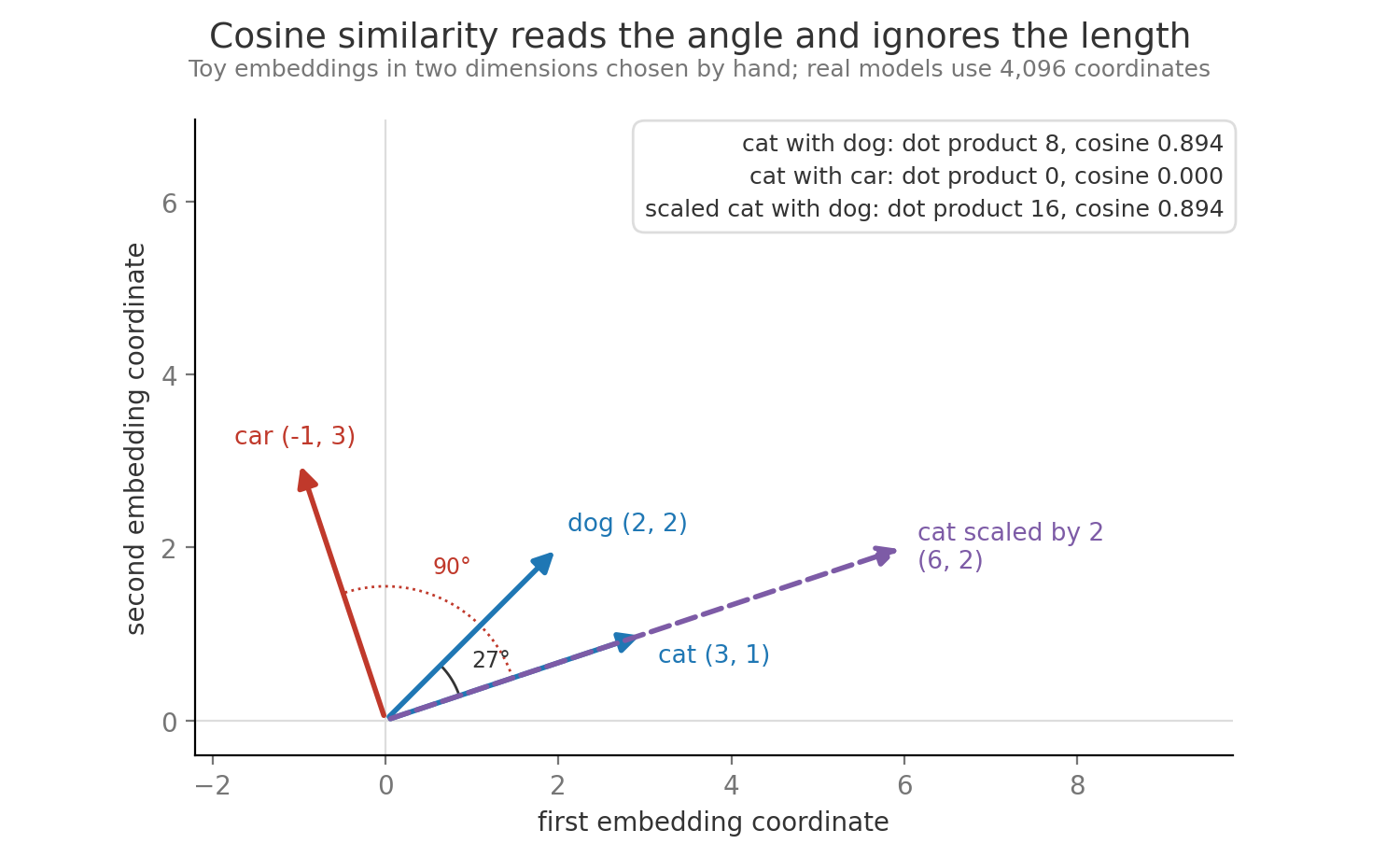
Training produces this geometry through the output scores. The logit for token is a dot product, , where is row of the output head . Tokens that are good continuations in the same contexts are pushed toward the same hidden vectors, so their rows drift toward each other, and cat and dog end up closer than cat and car. Trained tables are usually anisotropic. Anisotropy means most rows share a common direction, so two unrelated tokens often have a positive cosine such as 0.3, and a raw cosine has to be compared against that baseline before it means anything. Input embedding rows are a starting representation, and the vectors used for retrieval come from later layers (see Using LLMs in Applications).
10. Weight tying
Section titled “10. Weight tying”The embedding table and the output head do mirror image jobs. One turns a token id into a vector, the other scores how well a vector matches each token, and both are by matrices with one row per token. It is natural to ask whether the model needs two copies, the way one bilingual dictionary can be read in either direction.
Weight tying uses one matrix for both, so the output head is the embedding table, , and the logit for token becomes , the dot product of the final hidden vector with token ‘s own embedding. Press and Wolf showed that tying often improves language models at no extra cost, since every training step now updates the shared rows from both ends. In the reference model tying would save 131,072,000 parameters, about 1.9% of 6.74 billion and 262 MB of bfloat16 weights, and it saves no compute, since the head still multiplies by every row.
The saving matters more for small models and large vocabularies. A model of width 2,048 with 128,000 entries has 262,144,000 parameters in each table, about a quarter of a 1B model, so small models such as GPT-2 and Gemma tie, while Llama 2 7B keeps the two tables separate and lets the input and output roles specialize. The tradeoff and other forms of parameter sharing are developed in Efficient Parameter Sharing.
Related: Language Modeling and Next Token Prediction · Attention and Positional Information